

Preparing the dataset
In this chapter, we will build multiple ML models that will predict whether a hotel booking will be cancelled or not based on the information available. Hotel cancellations cause a lot of issues for hotel owners and managers, so trying to predict which reservations will be cancelled is a good use of our ML skills.
Before we start with our ML experiments, we will need a dataset that can be used when training our ML models. We will generate a realistic synthetic dataset similar to the Hotel booking demands dataset from Nuno Antonio, Ana de Almeida, and Luis Nunes.
The synthetic dataset will have a total of 21 columns. Here are some of the columns:
is_cancelled: Indicates whether the hotel booking was cancelled or notlead_time: [arrival date] – [booking date]adr: Average daily rateadults: Number of adultsdays_in_waiting_list: Number of days a booking stayed on the waiting list before getting confirmedassigned_room_type: The type of room that was assignedtotal_of_special_requests: The total number of special requests made by the customer
We will not discuss each of the fields in detail, but this should help us understand what data is available for us to use. For more information, you can find the original version of this dataset at https://www.kaggle.com/jessemostipak/hotel-booking-demand and https://www.sciencedirect.com/science/article/pii/S2352340918315191.
Generating a synthetic dataset using a deep learning model
One of the cool applications of ML would be having a deep learning model “absorb” the properties of an existing dataset and generate a new dataset with a similar set of fields and properties. We will use a pre-trained Generative Adversarial Network (GAN) model to generate the synthetic dataset.
Important note
Generative modeling involves learning patterns from the values of an input dataset, which are then used to generate a new dataset with a similar set of values. GANs are popular when it comes to generative modeling. For example, research papers have focused on how GANs can be used to generate “deepfakes,” where realistic images of humans are generated from a source dataset.
Generating and using a synthetic dataset has a lot of benefits, including the following:
- The ability to generate a much larger dataset than the original dataset that was used to train the model
- The ability to anonymize any sensitive information in the original dataset
- Being able to have a cleaner version of the dataset after data generation
That said, let’s start generating the synthetic dataset by running the following commands in the terminal of our Cloud9 environment (right after the $ sign at the bottom of the screen):
- Continuing from where we left off in the Installing the Python prerequisites section, run the following command to create an empty directory named
tmpin the current working directory:mkdir -p tmp
Note that this is different from the /tmp directory.
- Next, let’s download the
utils.pyfile using thewgetcommand:wget -O utils.py https://bit.ly/3CN4owx
The utils.py file contains the block() function, which will help us read and troubleshoot the logs generated by our scripts.
- Run the following command to download the pre-built GAN model into the Cloud9 environment:
wget -O hotel_bookings.gan.pkl https://bit.ly/3CHNQFT
Here, we have a serialized pickle file that contains the properties of the deep learning model.
Important note
There are a variety of ways to save and load ML models. One of the options would be to use the Pickle module to serialize a Python object and store it in a file. This file can later be loaded and deserialized back to a Python object with a similar set of properties.
- Create an empty
data_generator.pyscript file using thetouchcommand:touch data_generator.py
Important note
Before proceeding, make sure that the data_generator.py, hotel_bookings.gan.pkl, and utils.py files are in the same directory so that the synthetic data generator script works.
- Double-click the
data_generator.pyfile in the file tree (located on the left-hand side of the Cloud9 environment) to open the empty Python script file in the editor pane. - Add the following lines of code to import the prerequisites needed to run the script:
from ctgan import CTGANSynthesizer
from pandas_profiling import ProfileReport
from utils import block, debug
- Next, let’s add the following lines of code to load the pre-trained GAN model:
with block('LOAD CTGAN'): pkl = './hotel_bookings.gan.pkl' gan = CTGANSynthesizer.load(pkl) print(gan.__dict__) - Run the following command in the terminal (right after the
$sign at the bottom of the screen) to test if our initial blocks of code in the script are working as intended:python3 data_generator.py
This should give us a set of logs similar to what is shown in the following screenshot:
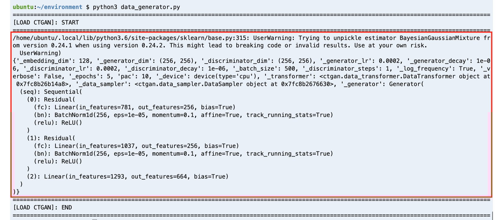
Figure 1.7 – GAN model successfully loaded by the script
Here, we can see that the pre-trained GAN model was loaded successfully using the CTGANSynthesizer.load() method. Here, we can also see what block (from the utils.py file we downloaded earlier) does to improve the readability of our logs. It simply helps mark the start and end of the execution of a block of code so that we can easily debug our scripts.
- Let’s go back to the editor pane (where we are editing
data_generator.py) and add the following lines of code:with block('GENERATE SYNTHETIC DATA'): synthetic_data = gan.sample(10000) print(synthetic_data)
When we run the script later, these lines of code will generate 10000 records and store them inside the synthetic_data variable.
- Next, let’s add the following block of code, which will save the generated data to a CSV file inside the
tmpdirectory:with block('SAVE TO CSV'): target_location = "tmp/bookings.all.csv" print(target_location) synthetic_data.to_csv( target_location, index=False ) - Finally, let’s add the following lines of code to complete the script:
with block('GENERATE PROFILE REPORT'):
    profile = ProfileReport(synthetic_data)
    target_location = "tmp/profile-report.html"
    profile.to_file(target_location)
This block of code will analyze the synthetic dataset and generate a profile report to help us analyze the properties of our dataset.
Important note
You can find a copy of the data_generator.py file here: https://github.com/PacktPublishing/Machine-Learning-Engineering-on-AWS/blob/main/chapter01/data_generator.py.
- With everything ready, let’s run the following command in the terminal (right after the
$sign at the bottom of the screen):python3 data_generator.py
It should take about a minute or so for the script to finish. Running the script should give us a set of logs similar to what is shown in the following screenshot:
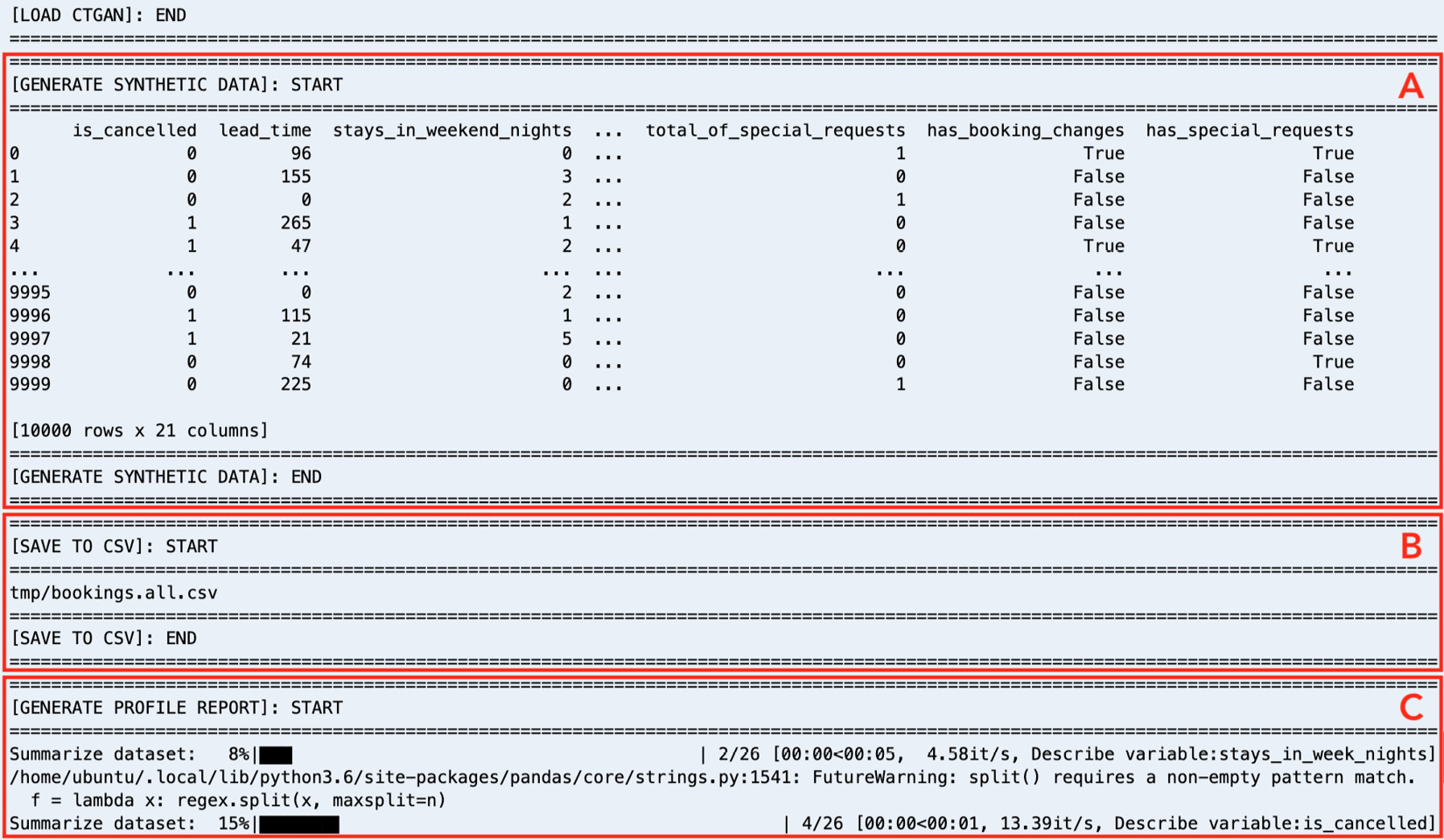
Figure 1.8 – Logs generated by data_generator.py
As we can see, running the data_generator.py script generates multiple blocks of logs, which should make it easy for us to read and debug what’s happening while the script is running. In addition to loading the CTGAN model, the script will generate the synthetic dataset using the deep learning model (A), save the generated data in a CSV file inside the tmp directory (tmp/bookings.all.csv) (B), and generate a profile report using pandas_profiling (C).
Wasn’t that easy? Before proceeding to the next section, feel free to use the file tree (located on the left-hand side of the Cloud9 environment) to check the generated files stored in the tmp directory.
Exploratory data analysis
At this point, we should have a synthetic dataset with 10000 rows. You might be wondering what our data looks like. Does our dataset contain invalid values? Do we have to worry about missing records? We must have a good understanding of our dataset since we may need to clean and process the data first before we do any model training work. EDA is a key step when analyzing datasets before they can be used to train ML models. There are different ways to analyze datasets and generate reports — using pandas_profiling is one of the faster ways to perform EDA.
That said, let’s check the report that was generated by the pandas_profiling Python library. Right-click on tmp/profile-report.html in the file tree (located on the left-hand side of the Cloud9 environment) and then select Preview from the list of options. We should find a report similar to the following:
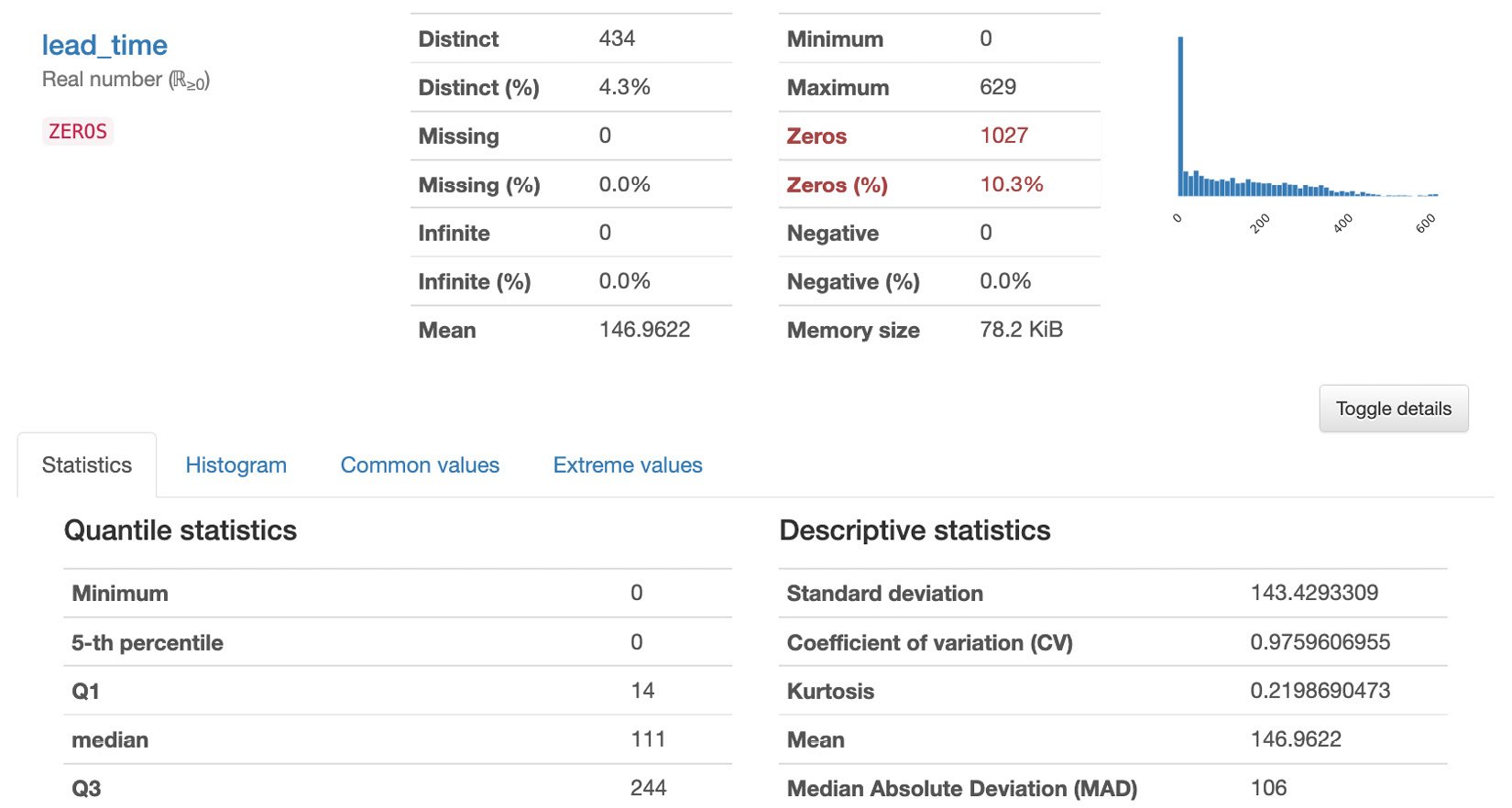
Figure 1.9 – Generated report
The report has multiple sections: Overview, Variables, Interactions, Correlations Missing Values, and Sample. In the Overview section, we can find a quick summary of the dataset statistics and the variable types. This includes the number of variables, number of records (observations), number of missing cells, number of duplicate rows, and other relevant statistics. In the Variables section, we can find the statistics and the distribution of values for each variable (column) in the dataset. In the Interactions and Correlations sections, we can see different patterns and observations regarding the potential relationship of the variables in the dataset. In the Missing values section, we can see if there are columns with missing values that we need to take care of. Finally, in the Sample section, we can see the first 10 and last 10 rows of the dataset.
Feel free to read through the report before proceeding to the next section.
Train-test split
Now that we have finished performing EDA, what do we do next? Assuming that our data is clean and ready for model training, do we just use all of the 10,000 records that were generated to train and build our ML model? Before we train our binary classifier model, we must split our dataset into training and test sets:
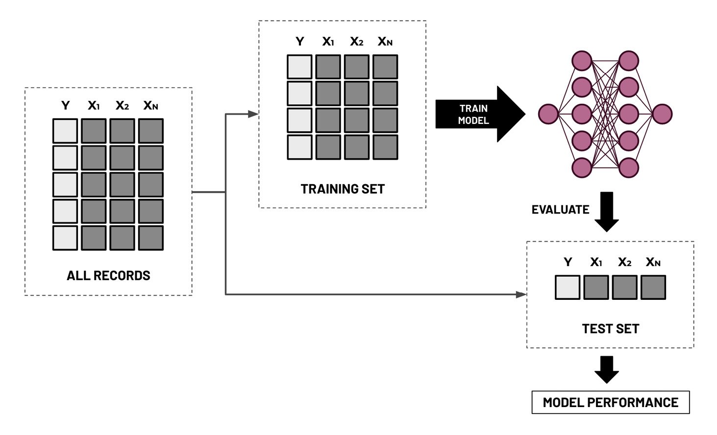
Figure 1.10 – Train-test split
As we can see, the training set is used to build the model and update its parameters during the training phase. The test set is then used to evaluate the final version of the model on data it has not seen before. What’s not shown here is the validation set, which is used to evaluate a model to fine-tune the hyperparameters during the model training phase. In practice, the ratio when dividing the dataset into training, validation, and test sets is generally around 60:20:20, where the training set gets the majority of the records. In this chapter, we will no longer need to divide the training set further into smaller training and validation sets since the AutoML tools and services will automatically do this for us.
Important note
Before proceeding with the hands-on solutions in this section, we must have an idea of what hyperparameters and parameters are. Parameters are the numerical values that a model uses when performing predictions. We can think of model predictions as functions such as y = m * x, where m is a parameter, x is a single predictor variable, and y is the target variable. For example, if we are testing the relationship between cancellations (y) and income (x), then m is the parameter that defines this relationship. If m is positive, cancellations go up as income goes up. If it is negative, cancellations lessen as income increases. On the other hand, hyperparameters are configurable values that are tweaked before the model is trained. These variables affect how our chosen ML models “model” the relationship. Each ML model has its own set of hyperparameters, depending on the algorithm used. These concepts will make more sense once we have looked at a few more examples in Chapter 2, Deep Learning AMIs, and Chapter 3, Deep Learning Containers.
Now, let’s create a script that will help us perform the train-test split:
- In the terminal of our Cloud9 environment (right after the
$sign at the bottom of the screen), run the following command to create an empty file calledtrain_test_split.py:touch train_test_split.py
- Using the file tree (located on the left-hand side of the Cloud9 environment), double-click the
train_test_split.pyfile to open the file in the editor pane. - In the editor pane, add the following lines of code to import the prerequisites to run the script:
import pandas as pd
from utils import block, debug
from sklearn.model_selection import train_test_split
- Add the following block of code, which will read the contents of a CSV file and store it inside a pandas
DataFrame:with block('LOAD CSV'): generated_df = pd.read_csv('tmp/bookings.all.csv') - Next, let’s use the
train_test_split()function from scikit-learn to divide the dataset we have generated into a training set and a test set:with block('TRAIN-TEST SPLIT'): train_df, test_df = train_test_split( generated_df, test_size=0.3, random_state=0 ) print(train_df) print(test_df) - Lastly, add the following lines of code to save the training and test sets into their respective CSV files inside the
tmpdirectory:with block('SAVE TO CSVs'): train_df.to_csv('tmp/bookings.train.csv', index=False) test_df.to_csv('tmp/bookings.test.csv', index=False)
Important note
You can find a copy of the train_test_split.py file here: https://github.com/PacktPublishing/Machine-Learning-Engineering-on-AWS/blob/main/chapter01/train_test_split.py.
- Now that we have completed our script file, let’s run the following command in the terminal (right after the
$sign at the bottom of the screen):python3 train_test_split.py
This should generate a set of logs similar to what is shown in the following screenshot:
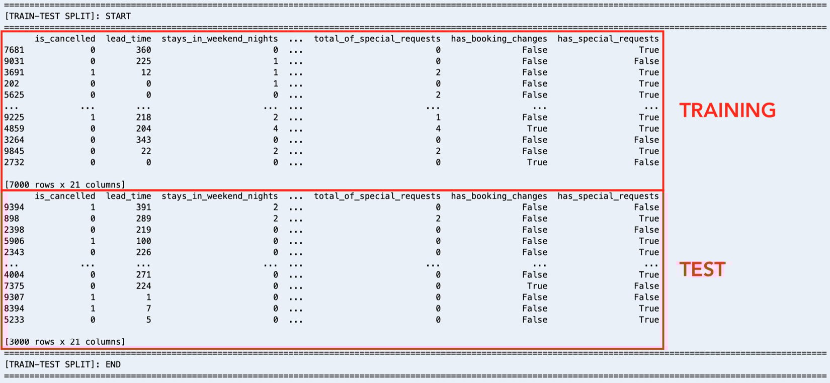
Figure 1.11 – Train-test split logs
Here, we can see that our training dataset contains 7,000 records, while the test set contains 3,000 records.
With this, we can upload our dataset to Amazon S3.
Uploading the dataset to Amazon S3
Amazon S3 is the object storage service for AWS and is where we can store different types of files, such as dataset CSV files and output artifacts. When using the different services of AWS, it is important to note that these services sometimes require the input data and files to be stored in an S3 bucket first or in a resource created using another service.
Uploading the dataset to S3 should be easy. Continuing where we left off in the Train-test split section, we will run the following commands in the terminal:
- Run the following commands in the terminal. Here, we are going to create a new S3 bucket that will contain the data we will be using in this chapter. Make sure that you replace the value of
<INSERT BUCKET NAME HERE>with a bucket name that is globally unique across all AWS users:BUCKET_NAME="<INSERT BUCKET NAME HERE>" aws s3 mb s3://$BUCKET_NAME
For more information on S3 bucket naming rules, feel free to check out https://docs.aws.amazon.com/AmazonS3/latest/userguide/bucketnamingrules.html.
- Now that the S3 bucket has been created, let’s upload the training and test datasets using the AWS CLI:
S3=s3://$BUCKET_NAME/datasets/bookings
TRAIN=bookings.train.csv
TEST=bookings.test.csv
aws s3 cp tmp/bookings.train.csv $S3/$TRAIN
aws s3 cp tmp/bookings.test.csv $S3/$TEST
Now that everything is ready, we can proceed with the exciting part! It’s about time we perform multiple AutoML experiments using a variety of solutions and services.