
AutoML with AutoGluon
Previously, we discussed what hyperparameters are. When training and tuning ML models, it is important for us to know that the performance of an ML model depends on the algorithm, the training data, and the hyperparameter configuration that’s used when training the model. Other input configuration parameters may also affect the performance of the model, but we’ll focus on these three for now. Instead of training a single model, teams build multiple models using a variety of hyperparameter configurations. Changes and tweaks in the hyperparameter configuration affect the performance of a model – some lead to better performance, while others lead to worse performance. It takes time to try out all possible combinations of hyperparameter configurations, especially if the model tuning process is not automated.
These past couple of years, several libraries, frameworks, and services have allowed teams to make the most out of automated machine learning (AutoML) to automate different parts of the ML process. Initially, AutoML tools focused on automating the hyperparameter optimization (HPO) processes to obtain the optimal combination of hyperparameter values. Instead of spending hours (or even days) manually trying different combinations of hyperparameters when running training jobs, we’ll just need to configure, run, and wait for this automated program to help us find the optimal set of hyperparameter values. For years, several tools and libraries that focus on automated hyperparameter optimization were available for ML practitioners for use. After a while, other aspects and processes of the ML workflow were automated and included in the AutoML pipeline.
There are several tools and services available for AutoML and one of the most popular options is AutoGluon. With AutoGluon, we can train multiple models using different algorithms and evaluate them with just a few lines of code:
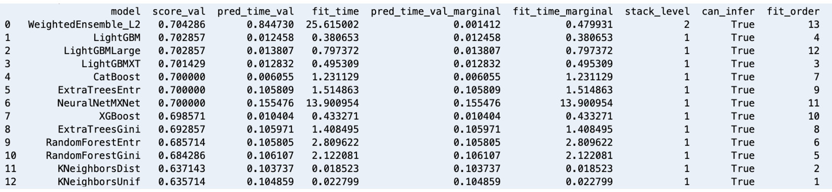
Figure 1.12 – AutoGluon leaderboard – models trained using a variety of algorithms
Similar to what is shown in the preceding screenshot, we can also compare the generated models using a leaderboard. In this chapter, we’ll use AutoGluon with a tabular dataset. However, it is important to note that AutoGluon also supports performing AutoML tasks for text and image data.
Setting up and installing AutoGluon
Before using AutoGluon, we need to install it. It should take a minute or so to complete the installation process:
- Run the following commands in the terminal to install and update the prerequisites before we install AutoGluon:
python3 -m pip install -U "mxnet<2.0.0"
python3 -m pip install numpy
python3 -m pip install cython
python3 -m pip install pyOpenSSL --upgrade
This book assumes that you are using the following versions or later: mxnet – 1.9.0, numpy – 1.19.5, and cython – 0.29.26.
- Next, run the following command to install
autogluon:python3 -m pip install autogluon
This book assumes that you are using autogluon version 0.3.1 or later.
Important note
This step may take around 5 to 10 minutes to complete. Feel free to grab a cup of coffee or tea!
With AutoGluon installed in our Cloud9 environment, let’s proceed with our first AutoGluon AutoML experiment.
Performing your first AutoGluon AutoML experiment
If you have used scikit-learn or other ML libraries and frameworks before, using AutoGluon should be easy and fairly straightforward since it uses a very similar set of methods, such as fit() and predict(). Follow these steps:
- To start, run the following command in the terminal:
ipython
This will open the IPython Read-Eval-Print-Loop (REPL)/interactive shell. We will use this similar to how we use the Python shell.
- Inside the console, type in (or copy) the following block of code. Make sure that you press Enter after typing the closing parenthesis:
from autogluon.tabular import (
    TabularDataset,
    TabularPredictor
)
- Now, let’s load the synthetic data stored in the
bookings.train.csvandbookings.test.csvfiles into thetrain_dataandtest_datavariables, respectively, by running the following statements:train_loc = 'tmp/bookings.train.csv' test_loc = 'tmp/bookings.test.csv' train_data = TabularDataset(train_loc) test_data = TabularDataset(test_loc)
Since the parent class of AutoGluon, TabularDataset, is a pandas DataFrame, we can use different methods on train_data and test_data such as head(), describe(), memory_usage(), and more.
- Next, run the following lines of code:
label = 'is_cancelled'
save_path = 'tmp'
tp = TabularPredictor(label=label, path=save_path)
predictor = tp.fit(train_data)
Here, we specify is_cancelled as the target variable of the AutoML task and the tmp directory as the location where the generated models will be stored. This block of code will use the training data we have provided to train multiple models using different algorithms. AutoGluon will automatically detect that we are dealing with a binary classification problem and generate multiple binary classifier models using a variety of ML algorithms.
Important note
Inside the tmp/models directory, we should find CatBoost, ExtraTreesEntr, and ExtraTreesGini, along with other directories corresponding to the algorithms used in the AutoML task. Each of these directories contains a model.pkl file that contains the serialized model. Why do we have multiple models? Behind the scenes, AutoGluon runs a significant number of training experiments using a variety of algorithms, along with different combinations of hyperparameter values, to produce the “best” model. The “best” model is selected using a certain evaluation metric that helps identify which model performs better than the rest. For example, if the evaluation metric that’s used is accuracy, then a model with an accuracy score of 90% (which gets 9 correct answers every 10 tries) is “better” than a model with an accuracy score of 80% (which gets 8 correct answers every 10 tries). That said, once the models have been generated and evaluated, AutoGluon simply chooses the model with the highest evaluation metric value (for example, accuracy) and tags it as the “best model.”
- Now that we have our “best model” ready, what do we do next? The next step is for us to evaluate the “best model” using the test dataset. That said, let’s prepare the test dataset for inference by removing the target label:
y_test = test_data[label]
test_data_no_label = test_data.drop(columns=[label])
- With everything ready, let’s use the
predict()method to predict theis_cancelledcolumn value of the test dataset provided as the payload:y_pred = predictor.predict(test_data_no_label)
- Now that we have the actual y values (
y_test) and the predicted y values (y_pred), let’s quickly check the performance of the trained model by using theevaluate_predictions()method:predictor.evaluate_predictions( y_true=y_test, y_pred=y_pred, auxiliary_metrics=True )
The previous block of code should yield performance metric values similar to the following:
{'accuracy': 0.691...,
 'balanced_accuracy': 0.502...,
 'mcc': 0.0158...,
 'f1': 0.0512...,
 'precision': 0.347...,
 'recall': 0.0276...}
In this step, we compare the actual values with the predicted values for the target column using a variety of formulas that compare how close these values are to each other. Here, the goal of the trained models is to make “the least number of mistakes” as possible over unseen data. Better models generally have better scores for performance metrics such as accuracy, Matthews correlation coefficient (MCC), and F1-score. We won’t go into the details of how model performance metrics work here. Feel free to check out https://bit.ly/3zn2crv for more information.
There’s more we can do using AutoGluon but this should help us appreciate how easy it is to use AutoGluon for AutoML experiments. There are other methods we can use, such as leaderboard(), get_model_best(), and feature_importance(), so feel free to check out https://auto.gluon.ai/stable/index.html for more information.