Neural networks for linear regression

In the preceding sections, we used mathematical expressions for calculating the coefficients of a linear regression equation. In this section, we will see how we can use the neural networks to perform the task of regression and build a neural network model using the TensorFlow Keras API.

Before performing regression using neural networks, let us first review what a neural network is. Simply speaking, a neural network is a network of many artificial neurons. From Chapter 1, Neural Network Foundations with TF, we know that the simplest neural network, the (simple) perceptron, can be mathematically represented as:

where f is the activation function. Consider, if we have f as a linear function, then the above expression is similar to the expression of linear regression that we learned in the previous section. In other words, we can say that a neural network, which is also called a function approximator, is a generalized regressor. Let us try to build a neural network simple regressor next using the TensorFlow Keras API.

Simple linear regression using TensorFlow Keras

In the first chapter, we learned about how to build a model in TensorFlow Keras. Here, we will use the same Sequential API to build a single-layered perceptron (fully connected neural network) using the Dense class. We will continue with the same problem, that is, predicting the price of a house given its area:

1. We start with importing the packages we will need. Notice the addition of the Keras module and the Dense layer in importing packages:

   import tensorflow as tf
   import numpy as np
   import matplotlib.pyplot as plt
   import pandas as pd
   import tensorflow.keras as K
   from tensorflow.keras.layers import Dense
   

2. Next, we generate the data, as in the previous case:

   #Generate a random data
   np.random.seed(0)
   area = 2.5 * np.random.randn(100) + 25
   price = 25 * area + 5 + np.random.randint(20,50, size = len(area))
   data = np.array([area, price])
   data = pd.DataFrame(data = data.T, columns=['area','price'])
   plt.scatter(data['area'], data['price'])
   plt.show()
   

3. The input to neural networks should be normalized; this is because input gets multiplied with weights, and if we have very large numbers, the result of multiplication will be large, and soon our metrics may cross infinity (the largest number your computer can handle):

   data = (data - data.min()) / (data.max() - data.min())  #Normalize
   

4. Let us now build the model; since it is a simple linear regressor, we use a Dense layer with only one unit:

   model = K.Sequential([
                         Dense(1, input_shape = [1,], activation=None)
   ])
   model.summary()
   

   Model: "sequential"
   ____________________________________________________________
    Layer (type)           Output Shape              Param #   
   ============================================================
    dense (Dense)          (None, 1)                 2         
                                                               
   ============================================================
   Total params: 2
   Trainable params: 2
   Non-trainable params: 0
   ____________________________________________________________
   

5. To train a model, we will need to define the loss function and optimizer. The loss function defines the quantity that our model tries to minimize, and the optimizer decides the minimization algorithm we are using. Additionally, we can also define metrics, which is the quantity we want to log as the model is trained. We define the loss function, optimizer (see Chapter 1, Neural Network Foundations with TF), and metrics using the compile function:

   model.compile(loss='mean_squared_error', optimizer='sgd')
   

6. Now that model is defined, we just need to train it using the fit function. Observe that we are using a batch_size of 32 and splitting the data into training and validation datasets using the validation_spilt argument of the fit function:

   model.fit(x=data['area'],y=data['price'], epochs=100, batch_size=32, verbose=1, validation_split=0.2)
   

   model.fit(x=data['area'],y=data['price'], epochs=100, batch_size=32, verbose=1, validation_split=0.2)
   Epoch 1/100
   3/3 [==============================] - 0s 78ms/step - loss: 1.2643 - val_loss: 1.4828
   Epoch 2/100
   3/3 [==============================] - 0s 13ms/step - loss: 1.0987 - val_loss: 1.3029
   Epoch 3/100
   3/3 [==============================] - 0s 13ms/step - loss: 0.9576 - val_loss: 1.1494
   Epoch 4/100
   3/3 [==============================] - 0s 16ms/step - loss: 0.8376 - val_loss: 1.0156
   Epoch 5/100
   3/3 [==============================] - 0s 15ms/step - loss: 0.7339 - val_loss: 0.8971
   Epoch 6/100
   3/3 [==============================] - 0s 16ms/step - loss: 0.6444 - val_loss: 0.7989
   Epoch 7/100
   3/3 [==============================] - 0s 14ms/step - loss: 0.5689 - val_loss: 0.7082
   .
   .
   .
   Epoch 96/100
   3/3 [==============================] - 0s 22ms/step - loss: 0.0827 - val_loss: 0.0755
   Epoch 97/100
   3/3 [==============================] - 0s 17ms/step - loss: 0.0824 - val_loss: 0.0750
   Epoch 98/100
   3/3 [==============================] - 0s 14ms/step - loss: 0.0821 - val_loss: 0.0747
   Epoch 99/100
   3/3 [==============================] - 0s 21ms/step - loss: 0.0818 - val_loss: 0.0740
   Epoch 100/100
   3/3 [==============================] - 0s 15ms/step - loss: 0.0815 - val_loss: 0.0740
   <keras.callbacks.History at 0x7f7228d6a790>
   

7. Well, you have successfully trained a neural network to perform the task of linear regression. The mean squared error after training for 100 epochs is 0.0815 on training data and 0.074 on validation data. We can get the predicted value for a given input using the predict function:

   y_pred = model.predict(data['area'])
   

8. Next, we plot a graph of the predicted and the actual data:

   plt.plot(data['area'], y_pred, color='red',label="Predicted Price")
   plt.scatter(data['area'], data['price'], label="Training Data")
   plt.xlabel("Area")
   plt.ylabel("Price")
   plt.legend()
   

9. Figure 2.3 shows the plot between the predicted data and the actual data. You can see that, just like the linear regressor, we have got a nice linear fit:

Figure 2.3: Predicted price vs actual price

10. In case you are interested in knowing the coefficients W and b, we can do it by printing the weights of the model using model.weights:

    [<tf.Variable 'dense/kernel:0' shape=(1, 1) dtype=float32, numpy=array([[-0.33806288]], dtype=float32)>,
    <tf.Variable 'dense/bias:0' shape=(1,) dtype=float32, numpy=array([0.68142694], dtype=float32)>]
    

We can see from the result above that our coefficients are W= 0.69 and bias b= 0.127. Thus, using linear regression, we can find a linear relationship between the house price and its area. In the next section, we explore multiple and multivariate linear regression using the TensorFlow Keras API.

Multiple and multivariate linear regression using the TensorFlow Keras API

The example in the previous section had only one independent variable, the area of the house, and one dependent variable, the price of the house. However, problems in real life are not that simple; we may have more than one independent variable, and we may need to predict more than one dependent variable. As you must have realized from the discussion on multiple and multivariate regression, they involve solving multiple equations. We can make our tasks easier by using the Keras API for both tasks.

Additionally, we can have more than one neural network layer, that is, we can build a deep neural network. A deep neural network is like applying multiple function approximators:

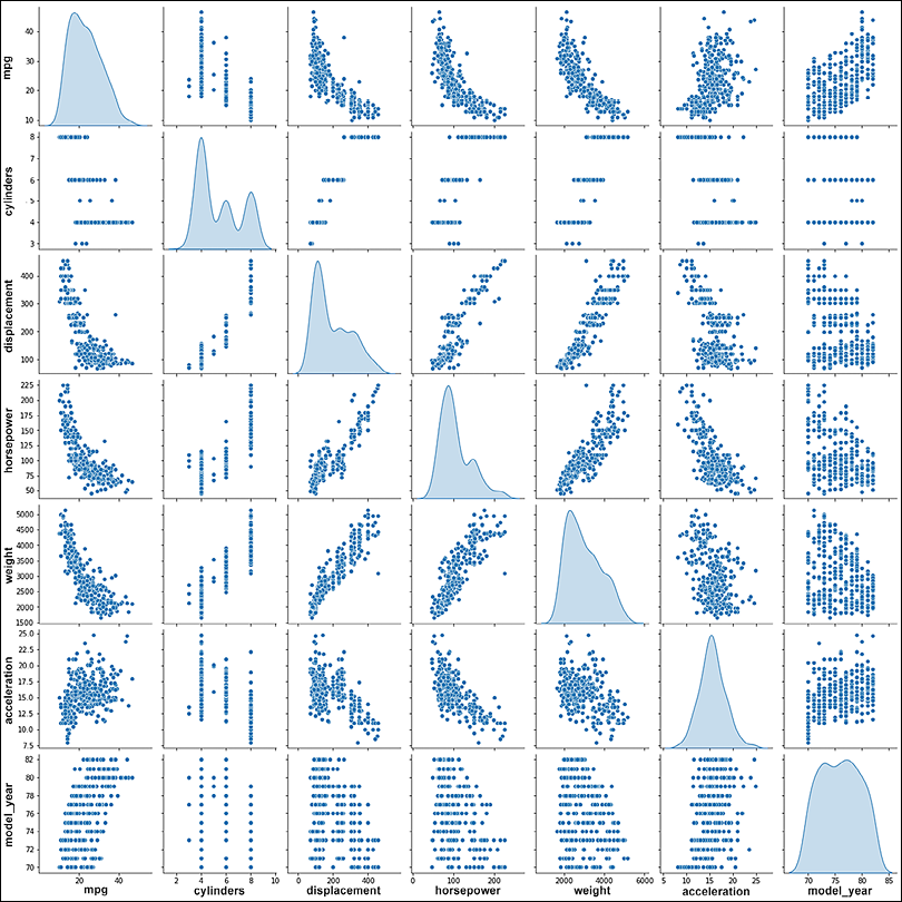
with being the function at layer L. From the expression above, we can see that if f was a linear function, adding multiple layers of a neural network was not useful; however, using a non-linear activation function (see Chapter 1, Neural Network Foundations with TF, for more details) allows us to apply neural networks to the regression problems where dependent and independent variables are related in some non-linear fashion. In this section, we will use a deep neural network, built using TensorFlow Keras, to predict the fuel efficiency of a car, given its number of cylinders, displacement, acceleration, and so on. The data we use is available from the UCI ML repository (Blake, C., & Merz, C. (1998), the UCI repository of machine learning databases (http://www.ics.uci.edu/~mlearn/MLRepository.html):

1. We start by importing the modules that we will need. In the previous example, we normalized our data using the DataFrame operations. In this example, we will make use of the Keras Normalization layer. The Normalization layer shifts the data to a zero mean and one standard deviation. Also, since we have more than one independent variable, we will use Seaborn to visualize the relationship between different variables:

   import tensorflow as tf
   import numpy as np
   import matplotlib.pyplot as plt
   import pandas as pd
   import tensorflow.keras as K
   from tensorflow.keras.layers import Dense, Normalization
   import seaborn as sns
   

2. Let us first download the data from the UCI ML repo.

   url = 'https://archive.ics.uci.edu/ml/machine-learning-databases/auto-mpg/auto-mpg.data'
   column_names = ['mpg', 'cylinders', 'displacement', 'horsepower', 'weight', 'acceleration', 'model_year', 'origin']
   data = pd.read_csv(url, names=column_names, na_values='?', comment='\t', sep=' ', skipinitialspace=True)
   

3. The data consists of eight features: mpg, cylinders, displacement, horsepower, weight, acceleration, model year, and origin. Though the origin of the vehicle can also affect the fuel efficiency “mpg” (miles per gallon), we use only seven features to predict the mpg value. Also, we drop any rows with NaN values:

   data = data.drop('origin', 1)
   print(data.isna().sum())
   data = data.dropna()
   

4. We divide the dataset into training and test datasets. Here, we are keeping 80% of the 392 datapoints as training data and 20% as test dataset:

   train_dataset = data.sample(frac=0.8, random_state=0)
   test_dataset = data.drop(train_dataset.index)
   

5. Next, we use Seaborn’s pairplot to visualize the relationship between the different variables:

   sns.pairplot(train_dataset[['mpg', 'cylinders', 'displacement','horsepower', 'weight', 'acceleration', 'model_year']], diag_kind='kde')
   

6. We can see that mpg (fuel efficiency) has dependencies on all the other variables, and the dependency relationship is non-linear, as none of the curves are linear:

Figure 2.4: Relationship among different variables of auto-mpg data

7. For convenience, we also separate the variables into input variables and the label that we want to predict:

   train_features = train_dataset.copy()
   test_features = test_dataset.copy() 
   train_labels = train_features.pop('mpg')
   test_labels = test_features.pop('mpg')
   

8. Now, we use the Normalization layer of Keras to normalize our data. Note that while we normalized our inputs to a value with mean 0 and standard deviation 1, the output prediction 'mpg' remains as it is:

   #Normalize
   data_normalizer = Normalization(axis=1)
   data_normalizer.adapt(np.array(train_features))
   

9. We build our model. The model has two hidden layers, with 64 and 32 neurons, respectively. For the hidden layers, we have used Rectified Linear Unit (ReLU) as our activation function; this should help in approximating the non-linear relation between fuel efficiency and the rest of the variables:

   model = K.Sequential([
       data_normalizer,
       Dense(64, activation='relu'),
       Dense(32, activation='relu'),
       Dense(1, activation=None)
   ])
   model.summary()
   

10. Earlier, we used stochastic gradient as the optimizer; this time, we try the Adam optimizer (see Chapter 1, Neural Network Foundations with TF, for more details). The loss function for the regression we chose is the mean squared error again:

    model.compile(optimizer='adam', loss='mean_squared_error')
    

11. Next, we train the model for 100 epochs:

    history = model.fit(x=train_features,y=train_labels, epochs=100, verbose=1, validation_split=0.2)
    

12. Cool, now that the model is trained, we can check if our model is overfitted, underfitted, or properly fitted by plotting the loss curve. Both validation loss and training loss are near each other as we increase the training epochs; this suggests that our model is properly trained:

    plt.plot(history.history['loss'], label='loss')
    plt.plot(history.history['val_loss'], label='val_loss')
    plt.xlabel('Epoch')
    plt.ylabel('Error [MPG]')
    plt.legend()
    plt.grid(True)
    

Figure 2.5: Model error

13. Let us finally compare the predicted fuel efficiency and the true fuel efficiency on the test dataset. Remember that the model has not seen a test dataset ever, thus this prediction is from the model’s ability to generalize the relationship between inputs and fuel efficiency. If the model has learned the relationship well, the two should form a linear relationship:

    y_pred = model.predict(test_features).flatten()
    a = plt.axes(aspect='equal')
    plt.scatter(test_labels, y_pred)
    plt.xlabel('True Values [MPG]')
    plt.ylabel('Predictions [MPG]')
    lims = [0, 50]
    plt.xlim(lims)
    plt.ylim(lims)
    plt.plot(lims, lims)
    

Figure 2.6: Plot between predicted fuel efficiency and actual values

14. Additionally, we can also plot the error between the predicted and true fuel efficiency:

    error = y_pred - test_labels
    plt.hist(error, bins=30)
    plt.xlabel('Prediction Error [MPG]')
    plt.ylabel('Count')
    

Figure 2.7: Prediction error

In case we want to make more than one prediction, that is, dealing with a multivariate regression problem, the only change would be that instead of one unit in the last dense layer, we will have as many units as the number of variables to be predicted. Consider, for example, we want to build a model which takes into account a student’s SAT score, attendance, and some family parameters, and wants to predict the GPA score for all four undergraduate years; then we will have the output layer with four units. Now that you are familiar with regression, let us move toward the classification tasks.