-
Book Overview & Buying

-
Table Of Contents

Deep Learning with TensorFlow and Keras – 3rd edition - Third Edition
By :
Deep Learning with TensorFlow and Keras – 3rd edition
By:
Overview of this book
Deep Learning with TensorFlow and Keras teaches you neural networks and deep learning techniques using TensorFlow (TF) and Keras. You'll learn how to write deep learning applications in the most powerful, popular, and scalable machine learning stack available.
TensorFlow 2.x focuses on simplicity and ease of use, with updates like eager execution, intuitive higher-level APIs based on Keras, and flexible model building on any platform. This book uses the latest TF 2.0 features and libraries to present an overview of supervised and unsupervised machine learning models and provides a comprehensive analysis of deep learning and reinforcement learning models using practical examples for the cloud, mobile, and large production environments.
This book also shows you how to create neural networks with TensorFlow, runs through popular algorithms (regression, convolutional neural networks (CNNs), transformers, generative adversarial networks (GANs), recurrent neural networks (RNNs), natural language processing (NLP), and graph neural networks (GNNs)), covers working example apps, and then dives into TF in production, TF mobile, and TensorFlow with AutoML.
Table of Contents (23 chapters)

Neural Network Foundations with TF
 Free Chapter
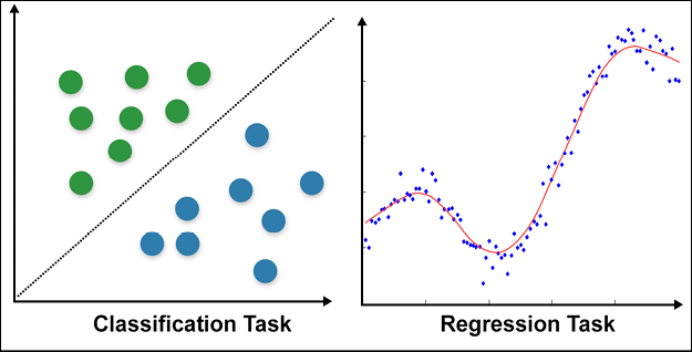
Regression and Classification
Convolutional Neural Networks
Word Embeddings
Recurrent Neural Networks
Transformers
Unsupervised Learning
Autoencoders
Generative Models
Self-Supervised Learning
Reinforcement Learning
Probabilistic TensorFlow
An Introduction to AutoML
The Math Behind Deep Learning
Tensor Processing Unit
Other Useful Deep Learning Libraries
Graph Neural Networks
Machine Learning Best Practices
TensorFlow 2 Ecosystem
Advanced Convolutional Neural Networks
Other Books You May Enjoy
Index

 and bias term b. In logistic regression, the coefficients are estimated using either the maximum likelihood estimator or stochastic gradient descent. If p is the total number of input data points, the loss is conventionally defined as a cross-entropy term given by: