Linear algebra, at its core, is about solving a set of linear equations, referred to as a system of equations. A large number of problems can be formulated as a system of linear equations.

We have two equations and two unknowns, as follows:

Both equations produce straight lines. The solution to both these equations is the point where both lines meet. In this case, the answer is the point (3, 1).

But for our purposes, in linear algebra, we write the preceding equations as a vector equation that looks like this:

Here, b is the result vector.

Placing the point (3, 1) into the vector equation, we get the following:

As we can see, the left-hand side is equal to the right-hand side, so it is, in fact, a solution! However, I personally prefer to write this as a coefficient matrix, like so:

Using the coefficient matrix, we can express the system of equations as a matrix problem in the form , where the column vector v is the variable vector. We write this as shown:

.

Going forward, we will express all our problems in this format.

To develop a better understanding, we'll break down the multiplication of matrix A and vector v. It is easiest to think of it as a linear combination of vectors. Let's take a look at the following example with a 3x3 matrix and a 3x1 vector:

It is important to note that matrix and vector multiplication is only possible when the number of columns in the matrix is equal to the number of rows (elements) in the vector.

For example, let's look at the following matrix:

This can be multiplied since the number of columns in the matrix is equal to the number of rows in the vector, but the following matrix cannot be multiplied as the number of columns and number of rows are not equal:

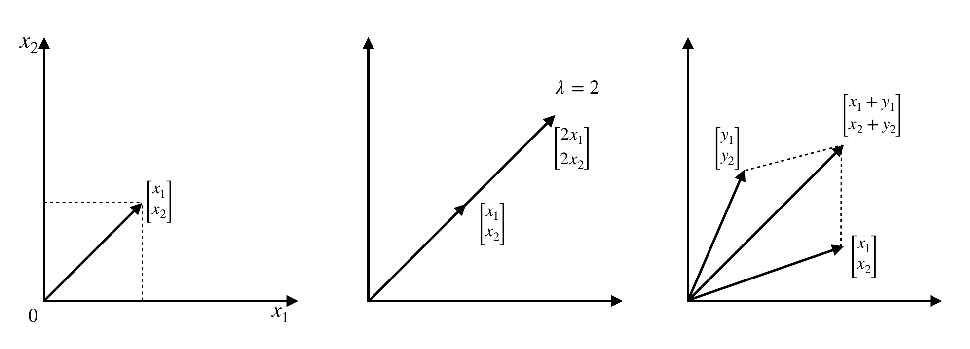
Let's visualize some of the operations on vectors to create an intuition of how they work. Have a look at the following screenshot:

The preceding vectors we dealt with are all in (in 2-dimensional space), and all resulting combinations of these vectors will also be in . The same applies for vectors in , , and .

There is another very important vector operation called the dot product, which is a type of multiplication. Let's take two arbitrary vectors in , v and w, and find its dot product, like this:

The following is the product:

.

Let's continue, using the same vectors we dealt with before, as follows:

And by taking their dot product, we get zero, which tells us that the two vectors are perpendicular (there is a 90° angle between them), as shown here:

The most common example of a perpendicular vector is seen with the vectors that represent the x axis, the y axis, and so on. In , we write the x axis vector as and the y axis vector as . If we take the dot product i•j, we find that it is equal to zero, and they are thus perpendicular.

By combining i and j into a 2x2 matrix, we get the following identity matrix, which is a very important matrix:

The following are some of the scenarios we will face when solving linear equations of the type :

• Let's consider the matrix and the equations and . If we do the algebra and multiply the first equation by 3, we get . But the second equation is equal to zero, which means that these two equations do not intersect and therefore have no solution. When one column is dependent on another—that is, is a multiple of another column—all combinations of and lie in the same direction. However, seeing as is not a combination of the two aforementioned column vectors and does not lie on the same line, it cannot be a solution to the equation.
• Let's take the same matrix as before, but this time, . Since b is on the line and is a combination of the dependent vectors, there is an infinite number of solutions. We say that b is in the column space of A. While there is only one specific combination of v that produces b, there are infinite combinations of the column vectors that result in the zero vector (0). For example, for any value, a, we have the following:

This leads us to another very important concept, known as the complete solution. The complete solution is all the possible ways to produce . We write this as , where .

Now that we've dealt with linear equations in 2-dimensions and have developed an understanding of them, let's go a step further and look at equations in 3-dimensions.

Earlier, our equations produced curves in the 2-dimensional space (xy-plane). Now, the equations we will be dealing with will produce planes in 3-dimensional space (xyz-plane).

Let's take an arbitrary 3x3 matrix, as follows:

We know from earlier in having dealt with linear equations in two dimensions that our solution b, as before, is a linear combination of the three column vectors, so that .

The equation (equation 1) produces a plane, as do (equation 2), and (equation 3).

When two planes intersect, they intersect at a line; however, when three planes intersect, they intersect at a point. That point is the vector , which is the solution to our problem.

However, if the three planes do not intersect at a point, there is no solution to the linear equation. This same concept of solving linear equations can be extended to many more dimensions.

Suppose now that we have a system with 15 linear equations and 15 unknown variables. We can use the preceding method and, according to it, we need to find the point that satisfies all the 15 equations—that is, where they intersect (if it exists).

It will look like this:

As you can tell, that's a lot of equations we have to deal with, and the greater the number of dimensions, the harder this becomes to solve.

One of the best ways to solve linear equations is by a systematic method known as elimination. This is a method that allows us to systematically eliminate variables and use substitution to solve equations.

Let's take a look at two equations with two variables, as follows:

After elimination, this becomes the following:

As we can see, the x variable is no longer in the second equation. We can plug the y value back into the first equation and solve for x. Doing this, we find that x = 3 and y = 1.

We call this triangular factorization. There are two types—lower triangular and upper triangular. We solve the upper triangular system from top to bottom using a process known as back substitution, and this works for systems of any size.

Let's solve three equations with three variables, as follows:

We will use upper triangular factorization and eliminate variables, starting with y and then z. Let's start by putting this into our matrix form, as follows:

For our purposes and to make things simpler, we will drop v, the column vector, and get the following result:

Then, exchange row 2 and row 3 with each other, like this:

Then, add row 2 and row 1 together to eliminate the first value in row 2, like this:

Next, multiply row 1 by 3/2 and subtract it from row 3, like this:

Finally, multiply row 2 by 6 and subtract it from row 3, like this:

As you can notice, the values in the matrix now form a triangle pointing upward, which is why we call it upper triangular. By substituting the values back into the previous equation backward (from bottom to top), we can solve, and find that , , and .

In summary, becomes , as illustrated here:

To check that our found solution is right, we solve , using our found values for x, y, and z, like this:

This then becomes the following equation:

And as we can see, the left-hand side is equal to the right-hand side.

After upper triangular factorization, an arbitrary 4x4 matrix will look like this:

We could take this a step further and factorize the upper triangular matrix until we end up with a matrix that contains only the pivot values along the diagonal, and zeros everywhere else. This resulting matrix P essentially fully solves the problem for us without us having to resort to forward or backward substitution, and it looks like this:

But as you can tell, there are a lot of steps involved in getting us from A to P.

There is one other very important factorization method called lower-upper (LU) decomposition. The way it works is we factorize A into an upper triangular matrix U, and record the steps of Gaussian elimination in a lower triangular matrix L, such that .

Let's revisit the matrix we upper-triangular factorized before and put it into LU factorized form, like this:

If we multiply the two matrices on the right, we will get the original matrix A. But how did we get here? Let's go through the steps, as follows:

1. We start with , so that the following applies:

2. We add -1 to what was the identity matrix at l_2,1 to represent the operation (row 2)-(-1)(row 1), so it becomes the following:

3. We then add to the matrix at l_3,1 to represent the operation, so it becomes the following:

4. We then add 6 to the matrix at l_3,2 to represent the operation (row 3)-6(row 2), so it becomes the following:

This is the LU factorized matrix we saw earlier.

You might now be wondering what this has to do with solving , which is very valid. The elimination process tends to work quite well, but we have to additionally apply all the operations we did on A to b as well, and this involves extra steps. However, LU factorization is only applied to A.

Let's now take a look at how we can solve our system of linear equations using this method.

For simplicity, we drop the variables vector and write A and b as follows:

But even this can get cumbersome to write as we go, so we will instead write it in the following way for further simplicity:

We then multiply both sides by and get the following result:

This tells us that , and we already know from the preceding equation that (so ). And by using back substitution, we can find the vector v.

In the preceding example, you may have noticed some new notation that I have not yet introduced, but not to worry—we will observe all the necessary notation and operations in the next section.